
Brazilian Electoral History
Overview
Recently, we are working on structuring data on the Brazilian Electoral History. I work at a Brazilian non-profit political school, called RenovaBR. We use data from the Brazilian Electoral History to develop analyzes and understand patterns between types of candidates.
In Brazil there is a public organization responsible for the elections, called TSE, that entity makes the data available as transparency to the population in a Data Repository. This data is available in CSV and TXT files, but without many standards. So we had the need to create a structure for this data and make ETL transformations, so that we can make analyzes from it.
We currently process data on brazilian elections for the following years: 2010, 2012, 2014, 2016, 2018. The full import of every year totals 26.151.069 million lines in the database.
So an architecture was created using the following technologies:
- Python - (Using pandas to read and transform data)
- MySQL - (Database)
- ELK - (Logstash, Elasticsearch, kibana)
The initial idea is to show the architecture and some queries, and in the next tutorial show some analysis using Elasticsearch and Kibana. With the data in Elasticsearch we created an API for querying and analyzing the data.
1. Project Architecture
Architecture used in the project:
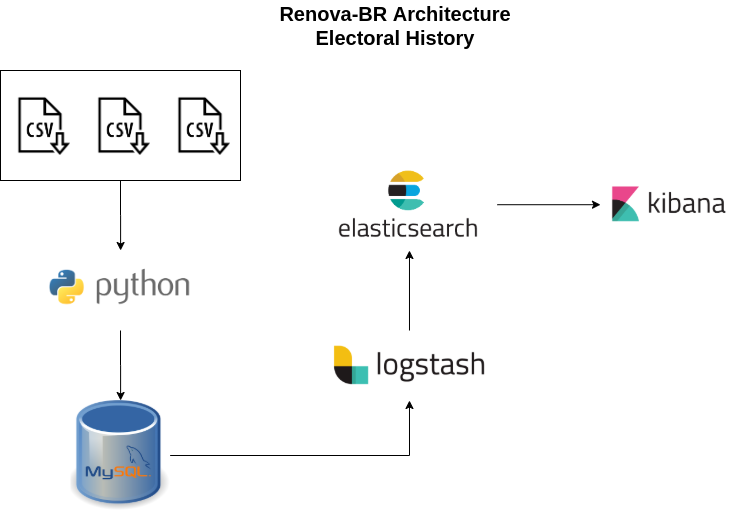
We decided to put the data first on MySQL, due to the ease of people on the team already using SQL language, then with Logstash we sent the data to Elasticsearch.
2. Processing the data
We automate the entire process to create the tables in the database and make the information available for analysis. To see the next-step to process the data check the page on the project that is publicly on GitHub:
https://github.com/renovabr/electoral-history
On a machine with 16 GB / 4 core, it takes around 10 hours to process all data.
3. Calculating the Electoral Coefficient
Also known as Hare Quote, it is a method by which the seats in the elections are distributed by the proportional system of votes in conjunction with the party quotient and the distribution of leftovers.
Elections in Brazil use the Brazilian proportional system to legislative seats. The program below calculates the electoral quotient for the 2016 year Brazilian Municipal Elections.
def main():
engine = create_engine(DATABASE, echo=False)
print('Read states. Wait...')
states = pd.read_sql(
"""SELECT sg_uf AS STATES FROM raw_tse_voting_cand_city WHERE election_year = '{}' GROUP BY 1""".format(YEAR),
engine)
output = 'result-quotient-' + YEAR + '.csv'
for st in states['STATES'].to_list():
print('Read votes: ' + st)
df0 = pd.read_sql("""
SELECT
sq_candidate AS SQ_CANDIDATO,
ds_position AS DS_CARGO,
cd_position AS CD_CARGO,
ds_situ_tot_shift AS DS_SIT_TOT_TURNO,
qt_votes_nominal AS QT_VOTOS_NOMINAIS,
nm_city AS NM_MUNICIPIO
FROM
raw_tse_voting_cand_city
WHERE
election_year = '{}'
AND sg_uf = '{}'""".format(YEAR, st), engine)
city = df0.groupby(['NM_MUNICIPIO'])
data = []
for name, group in city:
df1 = group.query(
"CD_CARGO == 13 and NM_MUNICIPIO == '" +
name +
"'").sort_values(
by=['QT_VOTOS_NOMINAIS'],
inplace=False,
ascending=False)
sigma1 = df1['QT_VOTOS_NOMINAIS'].sum()
elected = df1.query(
"DS_SIT_TOT_TURNO != 'SUPLENTE' and DS_SIT_TOT_TURNO != 'NÃO ELEITO' and DS_SIT_TOT_TURNO != '2º TURNO'")
sigma2 = elected.groupby(['SQ_CANDIDATO']).sum()
sigma2 = sigma2['QT_VOTOS_NOMINAIS'].count()
x = (sigma1 / sigma2)
q = np.ceil(x)
data.append([YEAR, st, name, q, sigma2])
df = pd.DataFrame(
data,
columns=[
'ANO_ELEICAO',
'SG_UF',
'NM_MUNICIPIO',
'Q_ELEITORAL',
'TOTAL_ELEITOS'])
if os.path.isfile(output):
df.to_csv(output, mode='a', index=False, sep=",", header=False)
else:
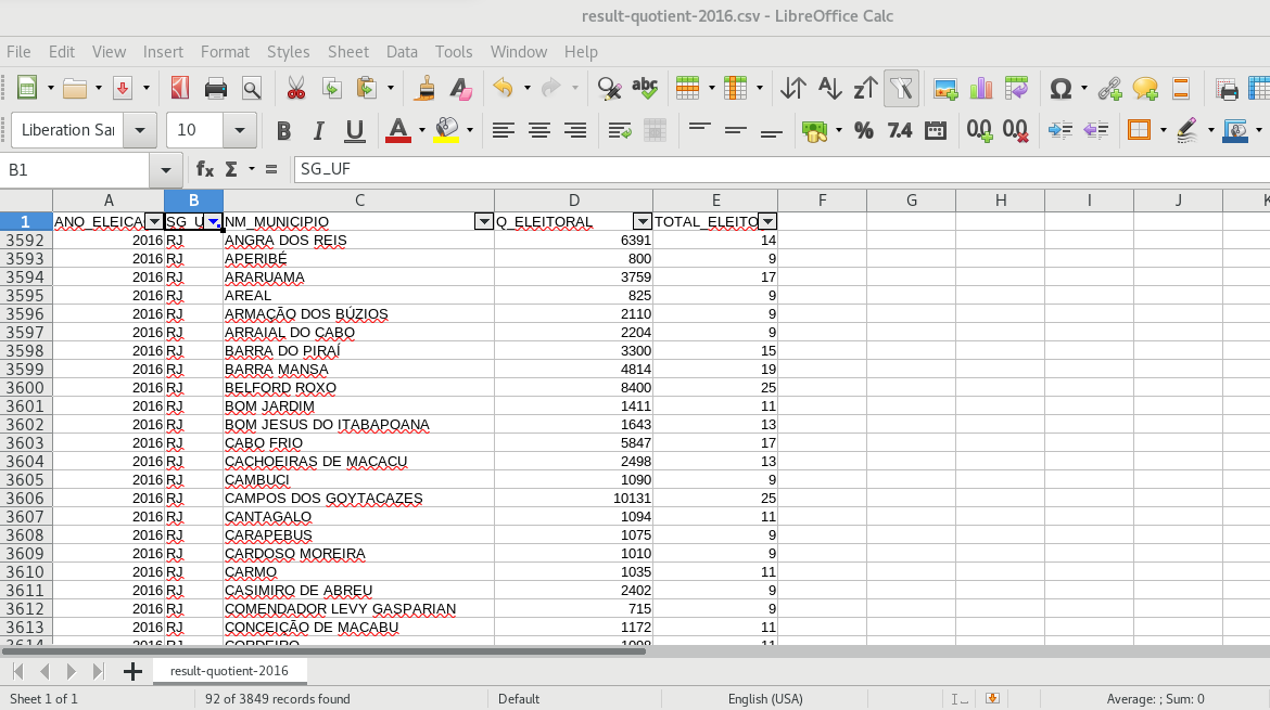
df.to_csv(output, index=False, sep=",")Check the complete code example here:
The result of the file, computing the electoral coefficient for all brazilian cities in the 2016 elections:
4. Some SQL queries
There is a data dictionary containing the description of the tables and fields:
Checking the total number of votes of the Governors of the state of Santa Catarina in the city of Florianópolis in the first shift of the 2018 elections.
SELECT
  sq_candidate AS SQ,
  nm_ballot_candidate AS Name,
  ds_position AS Position,
  nm_city AS City,
  format(sum(qt_votes_nominal), 0, 'de_DE') AS Votes
FROM
  raw_tse_voting_cand_city
WHERE
  election_year = '2018'
  AND sg_uf = 'SC'
  AND cd_city = 81051
  AND nr_shift = 1
  AND cd_position = 3
GROUP BY
  1,
  2,
  3,
  4
ORDER BY
  sum(qt_votes_nominal) DESC;
Result:
| SQ | Name | Position | City | Votes |
|---|---|---|---|---|
| 240000609724 | COMANDANTE MOISÉS | Governador | FLORIANÓPOLIS | 73.947 |
| 240000621321 | GELSON MERÍSIO | Governador | FLORIANÓPOLIS | 59.524 |
| 240000609537 | MAURO MARIANI | Governador | FLORIANÓPOLIS | 43.796 |
| 240000624336 | DÉCIO LIMA | Governador | FLORIANÓPOLIS | 39.144 |
| 240000601841 | CAMASÃO | Governador | FLORIANÓPOLIS | 19.362 |
| 240000616318 | PORTANOVA | Governador | FLORIANÓPOLIS | 4.844 |
| 240000610038 | INGRID ASSIS | Governador | FLORIANÓPOLIS | 1.644 |
| 240000614244 | JESSE PEREIRA | Governador | FLORIANÓPOLIS | 1.281 |
Checking the total number of votes of the Governors of the State of São Paulo in the first shift of the 2018 elections.
SELECT
  sq_candidate AS SQ,
  nm_ballot_candidate AS Name,
  ds_position AS Position,
  format(sum(qt_votes_nominal), 0, 'de_DE') AS Votes
FROM
  raw_tse_voting_cand_city
WHERE
  election_year = '2018'
  AND sg_uf = 'SP'
  AND nr_shift = 1
  AND cd_position = 3
GROUP BY
  1,
  2,
  3
ORDER BY
  sum(qt_votes_nominal) DESC;
Result:
| SQ | Name | Position | Votes |
|---|---|---|---|
| 250000612596 | JOÃO DORIA | Governador | 6.431.555 |
| 250000615141 | MARCIO FRANÇA | Governador | 4.358.998 |
| 250000604077 | PAULO SKAF | Governador | 4.269.865 |
| 250000623884 | LUIZ MARINHO | Governador | 2.563.922 |
| 250000612133 | MAJOR COSTA E SILVA | Governador | 747.462 |
| 250000601939 | ROGERIO CHEQUER | Governador | 673.102 |
| 250000615464 | RODRIGO TAVARES | Governador | 649.729 |
| 250000601522 | PROFESSORA LISETE | Governador | 507.236 |
| 250000617766 | PROF. CLAUDIO FERNANDO | Governador | 28.666 |
| 250000609174 | TONINHO FERREIRA | Governador | 16.202 |
Which top 10 city has the most votes for a distinguished candidate example the candidate (250000612596) to governor of the state of São Paulo, for the second shift.
SELECT
  nm_city AS City,
  sum(qt_votes_nominal) AS Votes
FROM
  raw_tse_voting_cand_city
WHERE
  election_year = '2018'
  AND sg_uf = 'SP'
  AND nr_shift = 2
  AND cd_position = 3
  AND sq_candidate = 250000612596
GROUP BY
  1
ORDER BY
  2 DESC LIMIT 10;
Result:
| City | Votes |
|---|---|
| SÃO PAULO | 2447309 |
| CAMPINAS | 315524 |
| GUARULHOS | 240825 |
| SÃO JOSÉ DOS CAMPOS | 232775 |
| SOROCABA | 207470 |
| SANTO ANDRÉ | 202125 |
| SÃO BERNARDO DO CAMPO | 196202 |
| OSASCO | 176109 |
| RIBEIRÃO PRETO | 166728 |
| JUNDIAÍ | 143028 |
5. Conclusion
The main objective of this article is to help people who want to study data from Brazil’s electoral system. It is possible to create several queries to explore the data for analysis. In the next article we show charts and queries using Elasticsearch and Kibana.
More details can be found in RenovaBR’s public repository:
6. Authors
- Darlan Dal-Bianco - darlan at renovabr.org
- Ederson Corbari - ederson at renovabr.org
Thanks!